---

Examples

Basic Example

Attaching the sample dataset:

library(survival)
data(tobin)

Estimating linear regression using tobit:

## consider these two models:
m1 <- survreg(Surv(durable, durable>0, type='left') ~ age + quant,
              data=tobin, dist='gaussian')

Summarize estimated paramters:

summary(m1)

## 
## Call:
## survreg(formula = Surv(durable, durable > 0, type = "left") ~ 
##     age + quant, data = tobin, dist = "gaussian")
##               Value Std. Error      z        p
## (Intercept) 15.1449    16.0795  0.942 3.46e-01
## age         -0.1291     0.2186 -0.590 5.55e-01
## quant       -0.0455     0.0583 -0.782 4.34e-01
## Log(scale)   1.7179     0.3103  5.536 3.10e-08
## 
## Scale= 5.57 
## 
## Gaussian distribution
## Loglik(model)= -28.9   Loglik(intercept only)= -29.5
##  Chisq= 1.1 on 2 degrees of freedom, p= 0.58 
## Number of Newton-Raphson Iterations: 3 
## n= 20

Setting values for the explanatory variables to their sample averages and simulating quantity of interest.

library(smargins)

m.sm <- smargins(m1, quant = seq(210, 280, 10))

summary(m.sm)

##   quant       mean       sd    median lower_2.5 upper_97.5
## 1   210 -0.6283012 2.725337 -0.606587 -5.878629   4.556931
## 2   220 -1.0615717 2.351930 -1.047042 -5.471870   3.446931
## 3   230 -1.4948423 2.077732 -1.541911 -5.590536   2.467526
## 4   240 -1.9281129 1.945160 -2.005974 -5.782240   1.919111
## 5   250 -2.3613834 1.982829 -2.456732 -6.280053   1.708785
## 6   260 -2.7946540 2.181938 -2.898043 -6.962013   1.678773
## 7   270 -3.2279245 2.504271 -3.267990 -7.778296   1.839742
## 8   280 -3.6611951 2.909155 -3.711762 -9.082322   2.153392

library(ggplot2)

ggplot(summary(m.sm), aes(x = quant, y = mean)) +
    geom_smooth(aes(ymin = lower_2.5, ymax = upper_97.5),
                stat = "identity")

## Warning: Ignoring unknown aesthetics: ymin, ymax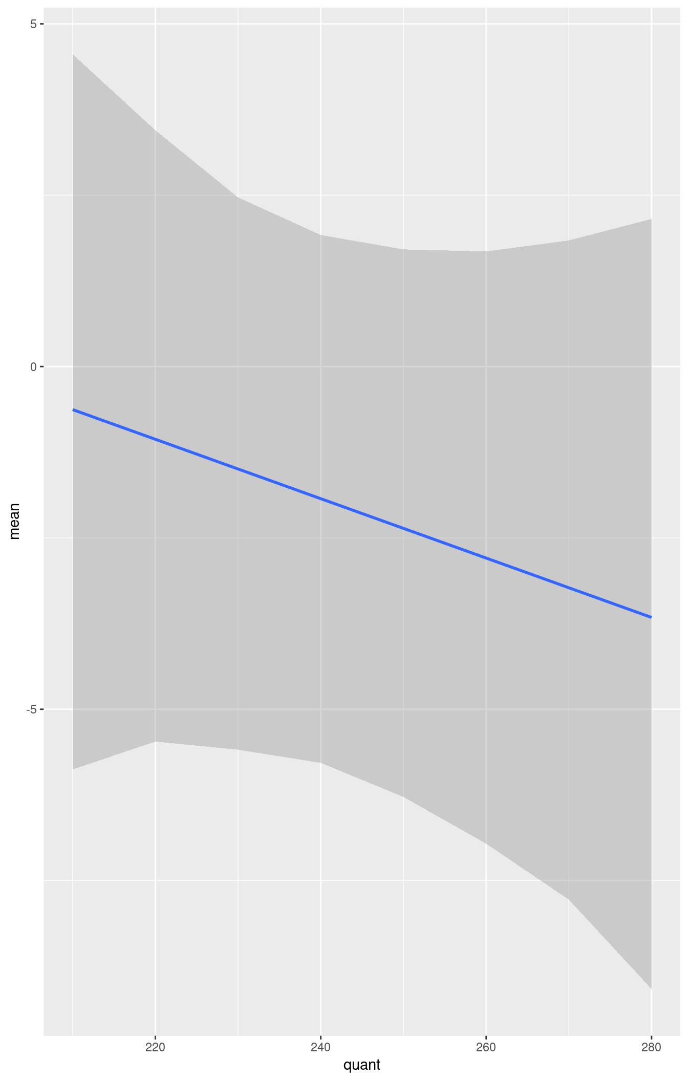

Simulating First Differences

Set explanatory variables to their default(mean/mode) values, with high (80th percentile) and low (20th percentile) liquidity ratio (quant):

m.sm2 <- smargins(m1, quant = quantile(tobin$quant, prob = c(0.2, 0.8)))

summary(m.sm2)

##   quant      mean       sd    median lower_2.5 upper_97.5
## 1 218.4 -1.004966 2.375453 -1.017309 -5.629625   3.476961
## 2 270.2 -3.311252 2.567358 -3.319656 -8.382085   1.743507

Estimating the first difference for the effect of high versus low liquidity ratio on duration( durable):

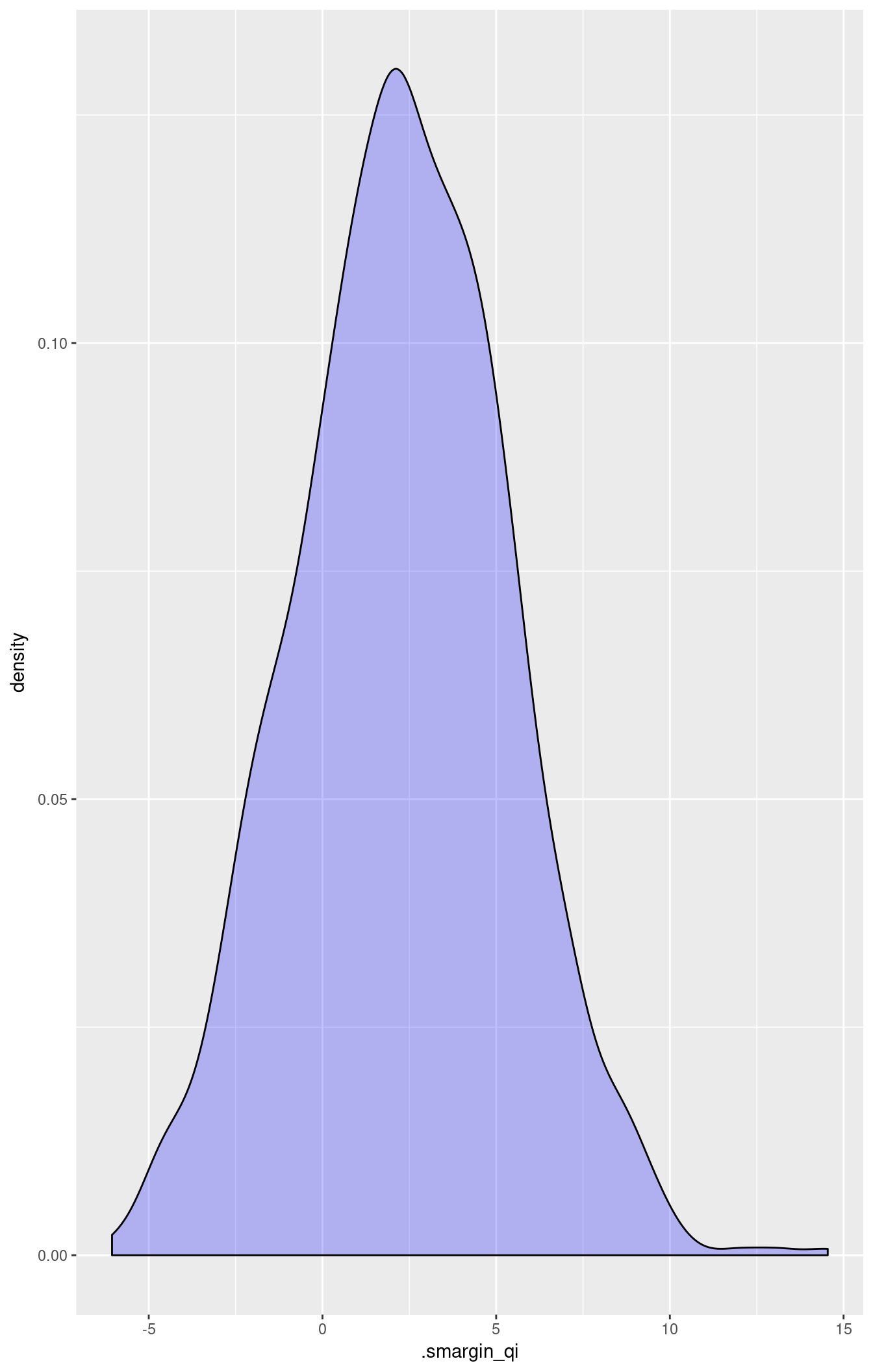
summary(scompare(m.sm2, "quant"))

##            quant     mean       sd   median lower_2.5 upper_97.5
## 1 218.4 vs 270.2 2.306287 3.043227 2.277627 -3.627821   8.411845

ggplot(scompare(m.sm2, "quant"), aes(x = .smargin_qi)) +
    geom_density(fill = "blue", alpha = 0.25)