---

Logit Regression for Dichotomous Dependent Variables with Survey Weights with logit.survey.

Use logit regression to model binary dependent variables specified as a function of a set of explanatory variables.

Examples

Example 1: User has Existing Sample Weights

Our example dataset comes from the survey package:

data(api, package = "survey")

In this example, we will estimate a model using the percentages of students who receive subsidized lunch and the percentage who are new to a school to predict whether each California public school attends classes year round. We first make a numeric version of the variable in the example dataset, which you may not need to do in another dataset.

library(survey)

## Loading required package: grid

## Loading required package: Matrix

## 
## Attaching package: 'survey'

## The following object is masked from 'package:graphics':
## 
##     dotchart

apistrat.design <- svydesign(ids = ~1, weights = ~pw, data = apistrat)

m1 <- svyglm(yr.rnd ~ meals + mobility,
             design = apistrat.design,
             family = quasibinomial())

summary(m1)

## 
## Call:
## svyglm(formula = yr.rnd ~ meals + mobility, design = apistrat.design, 
##     family = quasibinomial())
## 
## Survey design:
## svydesign(ids = ~1, weights = ~pw, data = apistrat)
## 
## Coefficients:
##             Estimate Std. Error t value Pr(>|t|)    
## (Intercept) -5.29981    0.97979  -5.409 1.82e-07 ***
## meals        0.03746    0.01158   3.235  0.00143 ** 
## mobility     0.06069    0.02001   3.032  0.00275 ** 
## ---
## Signif. codes:  0 '***' 0.001 '**' 0.01 '*' 0.05 '.' 0.1 ' ' 1
## 
## (Dispersion parameter for quasibinomial family taken to be 0.940999)
## 
## Number of Fisher Scoring iterations: 6

Set explanatory variables to their observed values, and set a high (80th percentile) and low (20th percentile) value for “meals,” the percentage of students who receive subsidized meals:

library(smargins)

m.sm1 <- smargins(m1, meals = quantile(meals, c(0.2, 0.8)))
summary(m.sm1)

##   meals       mean         sd     median   lower_2.5 upper_97.5
## 1  18.0 0.03161318 0.02207852 0.02562193 0.007244776 0.08909972
## 2  74.2 0.18169155 0.03941668 0.17847417 0.112966435 0.26736271

Generate first differences for the effect of high versus low “meals” on the probability that a school will hold classes year round:

m.sm1.diff <- scompare(m.sm1, "meals")
summary(m.sm1.diff)

##        meals       mean         sd     median  lower_2.5  upper_97.5
## 1 18 vs 74.2 -0.1500784 0.04000775 -0.1474838 -0.2328644 -0.07629612

Generate a second set of fitted values and a plot:

library(ggplot2)

ggplot(m.sm1.diff, aes(x = .smargin_qi)) +
    geom_density(fill = "blue", alpha = 0.25)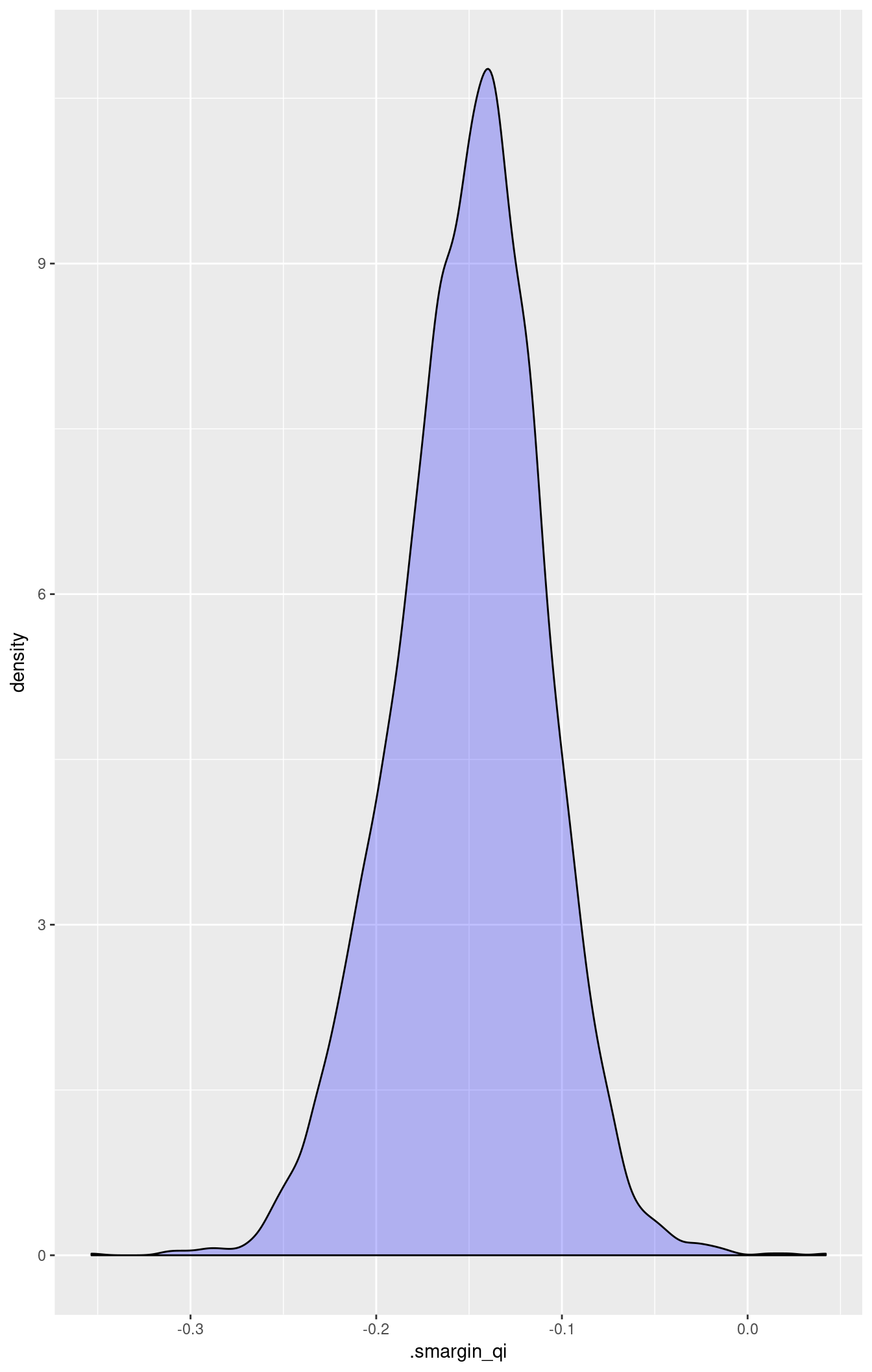

Example 2: User has Details about Complex Survey Design (but not sample weights)

Suppose that the survey house that provided the dataset excluded probability weights but made other details about the survey design available. We can still estimate a model without probability weights that takes instead variables that identify each the stratum and/or cluster from which each observation was selected and the size of the finite sample from which each observation was selected.

apiclus.design <- svydesign(ids = ~1, strata = ~stype, fpc = ~fpc, data = apistrat)

m2 <- svyglm(yr.rnd ~ meals + mobility,
             design = apiclus.design,
             family = quasibinomial())

summary(m2)

## 
## Call:
## svyglm(formula = yr.rnd ~ meals + mobility, design = apiclus.design, 
##     family = quasibinomial())
## 
## Survey design:
## svydesign(ids = ~1, strata = ~stype, fpc = ~fpc, data = apistrat)
## 
## Coefficients:
##             Estimate Std. Error t value Pr(>|t|)    
## (Intercept) -5.29981    0.96876  -5.471 1.36e-07 ***
## meals        0.03746    0.01145   3.270  0.00127 ** 
## mobility     0.06069    0.01929   3.145  0.00192 ** 
## ---
## Signif. codes:  0 '***' 0.001 '**' 0.01 '*' 0.05 '.' 0.1 ' ' 1
## 
## (Dispersion parameter for quasibinomial family taken to be 0.940999)
## 
## Number of Fisher Scoring iterations: 6

The coefficient estimates from this model are identical to point estimates in the previous example, but the standard errors are smaller.

m.sm2 <- smargins(m2, meals = quantile(apistrat$meals, c(0.2, 0.8)))
summary(m.sm2)

##   meals       mean         sd     median   lower_2.5 upper_97.5
## 1  18.0 0.03127663 0.02207439 0.02584485 0.006952182 0.08708536
## 2  74.2 0.18148118 0.03959123 0.17758124 0.113059958 0.27000292