Examples

Basic example

Attach the sample turnout dataset:

data(turnout, package = "Zelig")

Estimating parameter values for the logistic regression:

m1 <- glm(vote ~ age + race, family = binomial(link = "logit"), data = turnout)

Summarize estimated parameters:

summary(m1)

## 
## Call:
## glm(formula = vote ~ age + race, family = binomial(link = "logit"), 
##     data = turnout)
## 
## Deviance Residuals: 
##     Min       1Q   Median       3Q      Max  
## -1.9268  -1.2962   0.7072   0.7766   1.0723  
## 
## Coefficients:
##             Estimate Std. Error z value Pr(>|z|)    
## (Intercept) 0.038365   0.176920   0.217 0.828325    
## age         0.011263   0.003053   3.689 0.000225 ***
## racewhite   0.645551   0.134482   4.800 1.58e-06 ***
## ---
## Signif. codes:  0 '***' 0.001 '**' 0.01 '*' 0.05 '.' 0.1 ' ' 1
## 
## (Dispersion parameter for binomial family taken to be 1)
## 
##     Null deviance: 2266.7  on 1999  degrees of freedom
## Residual deviance: 2228.8  on 1997  degrees of freedom
## AIC: 2234.8
## 
## Number of Fisher Scoring iterations: 4

For logit models you may wish to calculate odds ratios:

cbind(OR = exp(coef(m1)), exp(confint(m1)))

## Waiting for profiling to be done...

##                   OR     2.5 %   97.5 %
## (Intercept) 1.039111 0.7347714 1.470780
## age         1.011327 1.0053346 1.017445
## racewhite   1.907038 1.4622538 2.478341

Set values for the explanatory variables and simulate quantities of interest from the posterior distribution:

library(smargins)
m.sm <- smargins(m1, age = 36, race = "white")
summary(m.sm)

##   age  race      mean        sd   median lower_2.5 upper_97.5
## 1  36 white 0.6088467 0.0290506 0.608863 0.5507057  0.6641614

Show the results graphically:

library(ggplot2)

ggplot(m.sm, aes(x = .smargin_qi)) +
    geom_density(aes(fill = interaction(age, race)))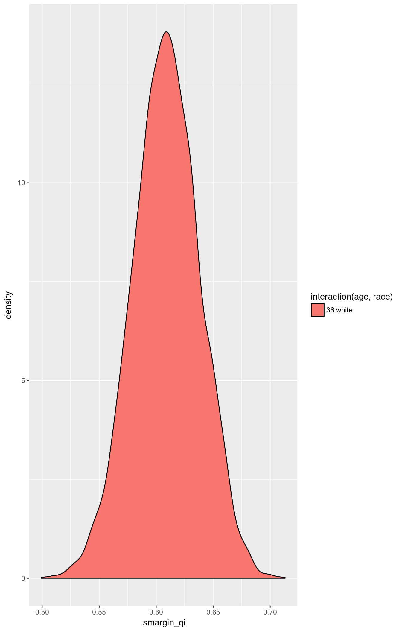

First differences

Estimating the risk difference (and risk ratio) between low education (25th percentile) and high education (75th percentile) while all the other variables averaged over their observed values.

m2 <- glm(vote ~ educate, data = turnout, family = binomial(link = "logit"))
m2.sm <- smargins(m2, educate = quantile(educate, prob = c(0.25, 0.75)))

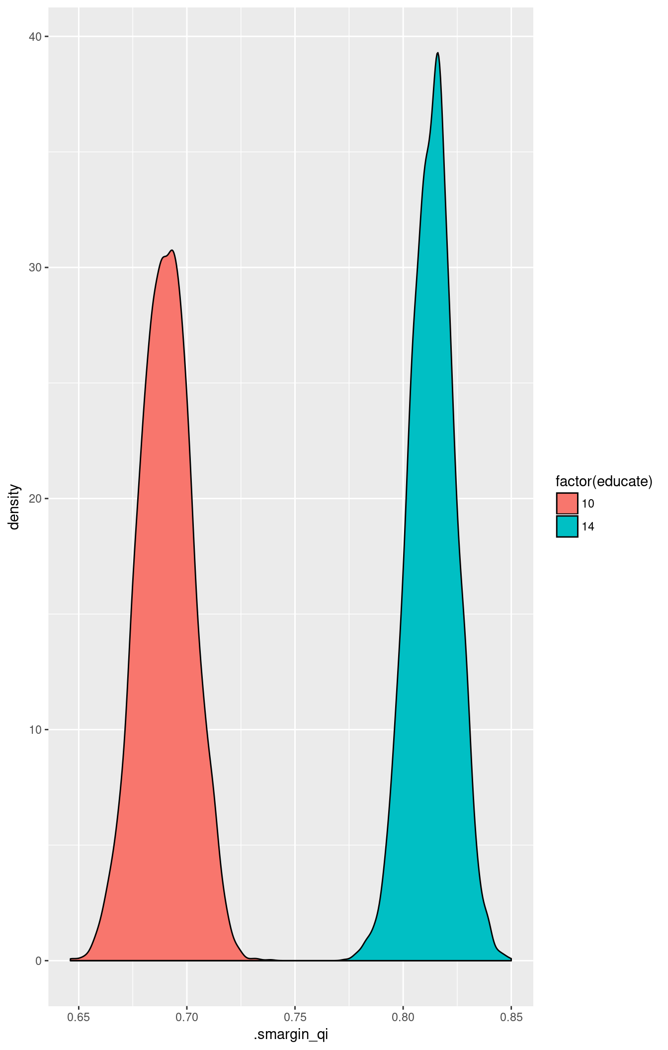
summary(m2.sm)

##   educate      mean         sd    median lower_2.5 upper_97.5
## 1      10 0.6901043 0.01221313 0.6901476 0.6659910  0.7134331
## 2      14 0.8132709 0.01045084 0.8136569 0.7927545  0.8332865

summary(scompare(m2.sm, var = "educate"))

##    educate       mean         sd     median  lower_2.5 upper_97.5
## 1 10 vs 14 -0.1231666 0.01165802 -0.1231291 -0.1461423 -0.1000393

ggplot(scompare(m2.sm, "educate")) +
    geom_density(aes(x = .smargin_qi, fill = factor(educate)))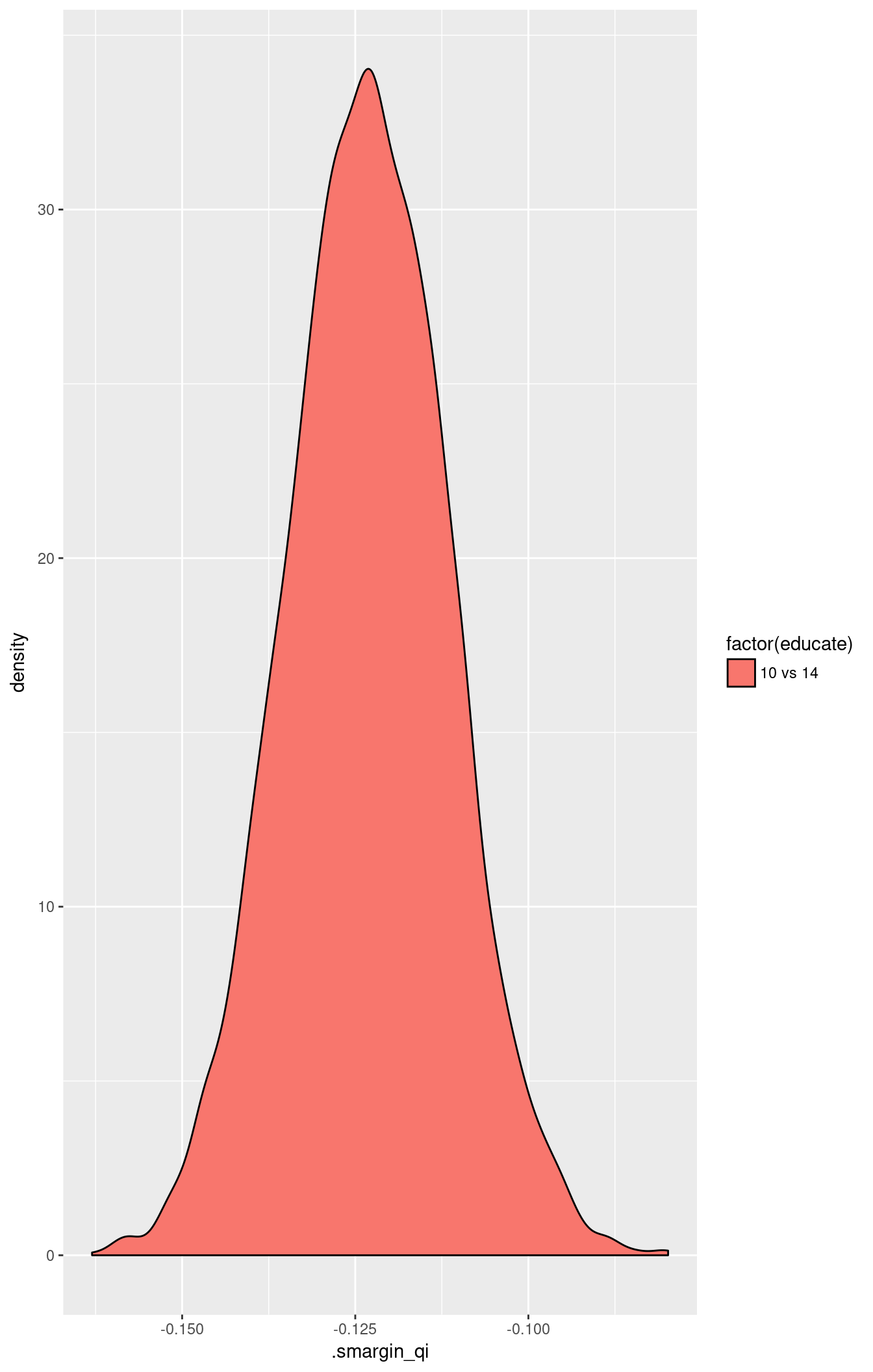

ggplot(m2.sm, aes(x = .smargin_qi)) +
    geom_density(aes(fill = factor(educate)))